Walkthrough: Spreadsheet basics
Total suggested time: 30 minutes
Now that you know more about the structure of a spreadsheet, we’ll explore the basic functionality of a spreadsheet program, including sorting, filtering and basic formulas.
Jump to a section
- Download the data
- Import the file
- Data dictionary
- Navigating the spreadsheet
- Sorting and filtering
- Functions and cell references
- Cleaning data with functions
- Filling down
- Adding data with formulas
- Nesting formulas
- Pasting ‘values only’
Download the data
We’ll be working with a simplified version of the COVID Tracking Project’s data on the state of New York using Google Sheets. Get started by downloading the CSV file below.
Import the file
In a new browser tab, open a new Google Sheet by typing sheet.new in the address bar.
Click where it says “Untitled Spreadsheet” and give it a name, then move it somewhere in your Google Drive where you can find it again.

You can name it anything you want – in our case, we’ll keep it simple and use covid_ny.
To import the file, click File > Import in the main menu, then click UPLOAD. From here, you’ll need to browse to where you downloaded your CSV file and select it or drag the file directly into the dialogue box.
Specifying Separator type gives us some control over how Sheets determines the column types in your data. But we can leave this alone for now.
Use the dropdown menu to change the Import location to “Replace spreadsheet,” then click OK.
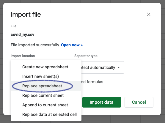
Sheets will process the file, and you should see your data!
Data dictionary
Take a minute to examine the data and think about the fields. Most are self-explanatory. Some less so.
Here’s the listing from the COVID Tracking Project’s field definitions, a data dictionary that tells us what each column means.
date- date on which data was collected by The COVID Tracking Projectstate- two-letter abbreviation for the state or territoryfips- Federal Information Processing System (FIPS) code for reporting statepositive- total number of confirmed plus probable cases of COVID-19 reported by the state or territorytotalTestResults- Total number of people tested per day via PCR testing as reported by the state or territoryhospitalizedCurrently- Individuals who are currently hospitalized with COVID-19inIcuCurrently- individuals who are currently hospitalized in the intensive care unit with COVID-19onVentilatorCurrently- individuals who are currently hospitalized under advanced ventilation with COVID-19death- total fatalities with confirmed OR probable COVID-19 case diagnosis
Navigating the spreadsheet
For sanity’s sake, let’s freeze the header row – where our column names are – by clicking View > Freeze > 1 row or by using the cursor to click and drag the thick grey bar in the top corner of our spreadsheet data. Now no matter where we scroll, we know what our columns mean.
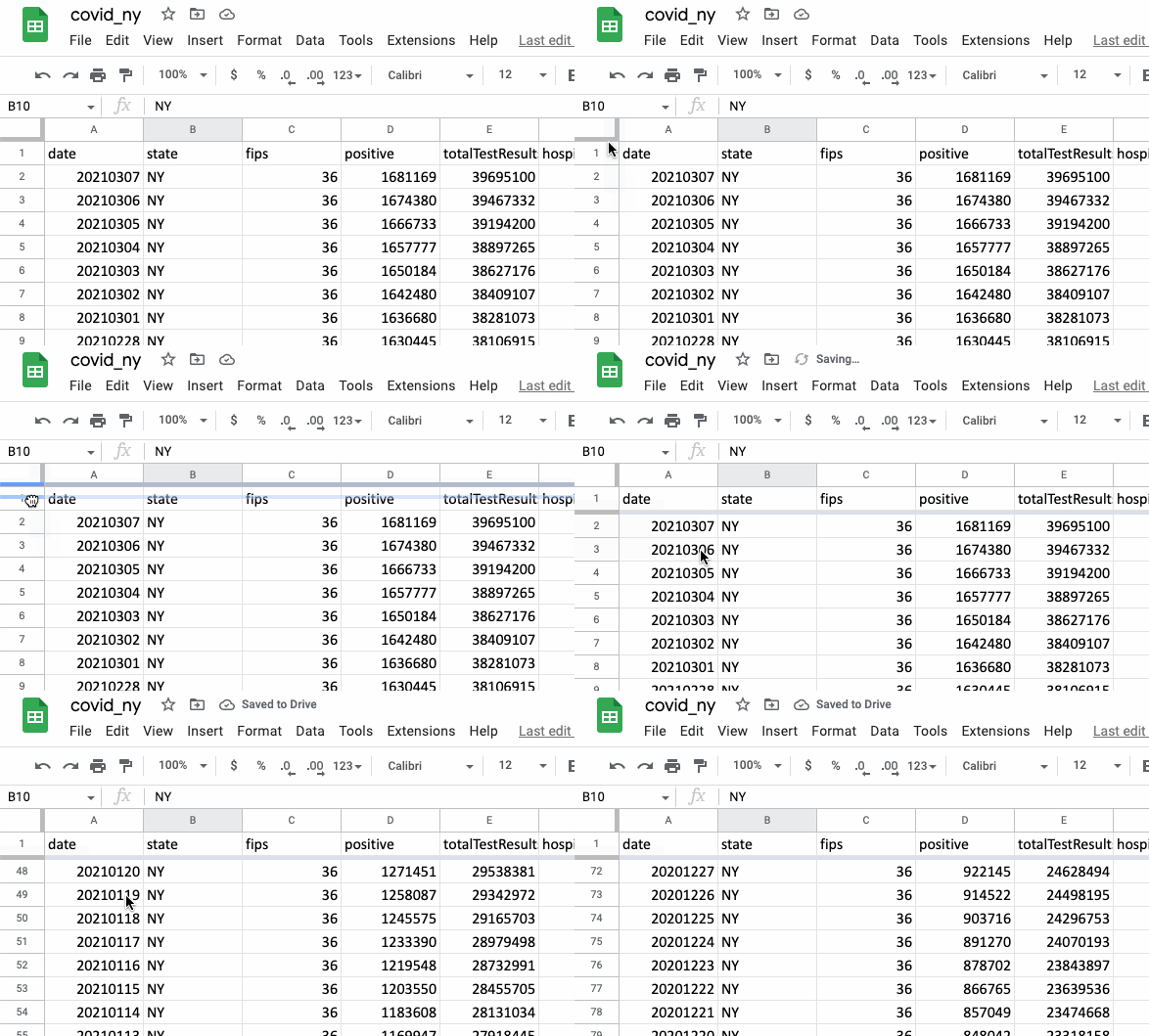
There’s a good bit of data here, and although it’s not impossible to scroll up and down through more than 300 rows, you could imagine this would get tedious if your data was 1,000 or 10,000 rows long.
To make our lives a little easier, we can use a series of keyboard shortcuts to navigate quickly around the sheet.
Pressing CTRL + ↓ (PC) or CMD + ↓ (Mac), for example, will jump down to the end of your current column – or the last cell with actual data in it. CTRL + ↑ / CMD + ↑ will jump back up to your header row.
Sorting and filtering
By default, the data is sorted by date in descending order. Let’s start from the beginning instead.
On the spreadsheet toolbar, you should see a button that looks like a funnel.

This is your filter toggle, and if you click it, you’ll notice a subtle change in your headers. They now have little inverted pyramids next to them!
In the date column, click the pyramid to bring up the filter dialogue, then click Sort A → Z.
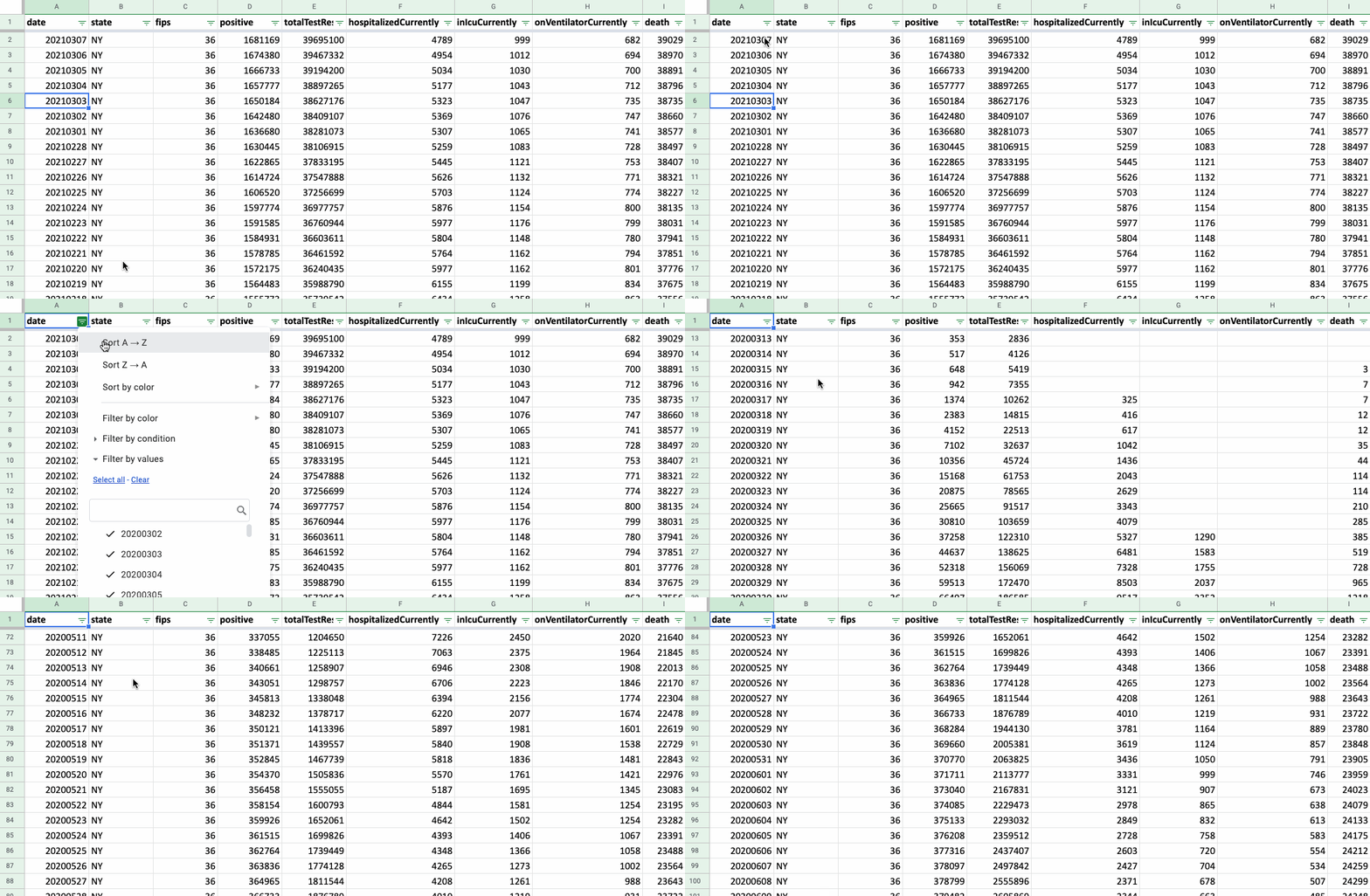
You’ll probably notice here that the “dates” don’t really look like dates – they’re actually numerics. But we’ll deal with that later. But if we think about it, we can see that 20200302 translates to “March 2, 2020,” the first day data was captured for New York (and about a week before the World Health Organization declared COVID-19 a pandemic).
We can also filter our data by condition, setting a criteria all rows must meet before they’re displayed.
For example, let’s see how many days saw more than 1,000 people on ventilators.
Click the pyramid next to the onVentilatorCurrently column to bring up the filter dialogue, then:
- Click
Filter by condition - Select
Greater than - Type
1000 - Click
OK
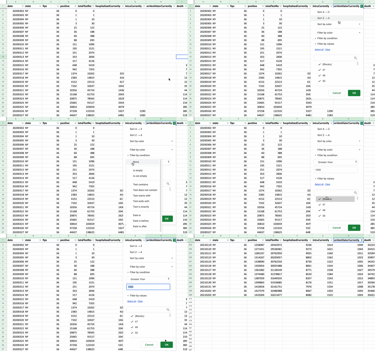
How many rows is that?
Find out by highlighting one of your columns (try onVentilatorCurrently). You’ll see a box pop up in the bottom right with a Sum value that isn’t all that helpful. Click the box to select Count Numbers instead (you can also use Count, although this will include the header row).
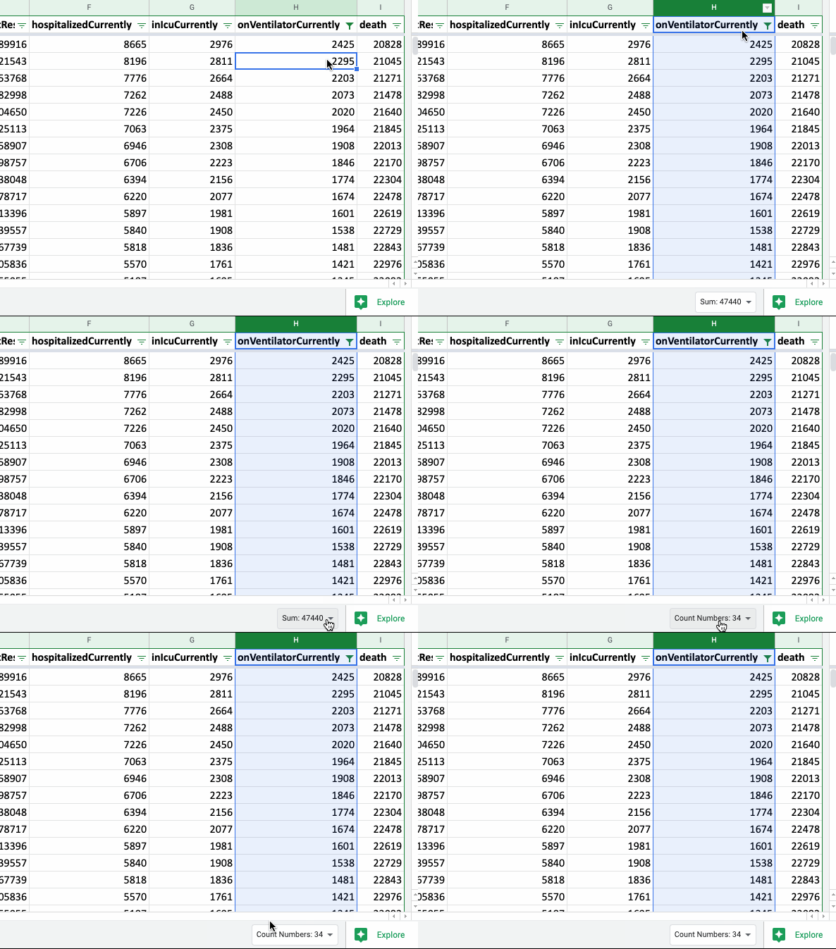
From there, we can see that 34 days saw more than 1,000 COVID-19 patients on ventilators.
Functions and cell references
Typing the equal sign at the beginning of the text string is an indicator to the spreadsheet software that some kind of formula follows (maybe just =2+2).
But spreadsheet software like Sheets has a set of built-in functions that perform some action based on the arguments they receive. In Excel, Sheets and just about any other spreadsheets software, a function looks like this:
=FUNCTION(argument1,argument2)
Arguments are contained in parentheses, and if there is more than one, they’re separated by commas.
There are functions to do basic math (SUM) and parse strings (FIND) and much more, each of which requires different arguments.
SUM, for example, just adds up all the arguments – and you can include as many as you want. The formula itself, once you type it, will only be visible in the function bar right about the spreadsheet. The data itself will show you the value returned by the function.
So =SUM(2,2) would display 4, and it’s the equivalent of just typing =4+4 in the cell.
Once you type = at the beginning of a cell, you can substitute values from other cells with a cell reference, a letter and number combination describing the row and column of the cell.
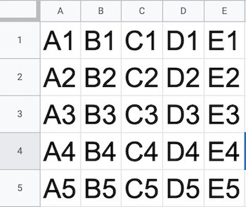
But you don’t actually need to look up a cell reference and hand-type it into a cell – once you begin a cell with an equal sign, you click on the cell you want and Sheets will insert the cell reference for you.
Cleaning data with formulas
We noted before that our “date” field isn’t quite right. In this case, Sheets has interpreted that column as a numeric value. So let’s practice a little data cleaning to get it right.
Start by toggling your filters off. You should be looking at all your original data – nothing hidden here.
Create a column by right-clicking on the A label of the data column, then clicking Insert 1 column right. Do this three times more to create four total new empty columns. We’ll name them year, month, day and date_clean.
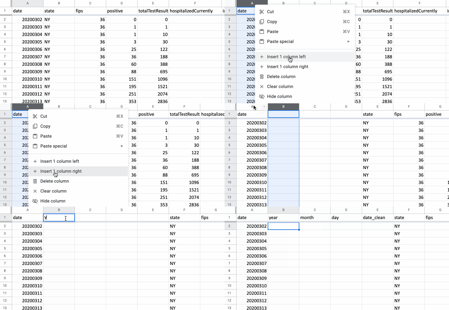
What we want to do is slice up the sequence of numbers in our date column. We’ll do that with a few functions designed exactly for that purpose: LEFT, MID and RIGHT.
Let’s tackle LEFT and RIGHT first.
=LEFT(string, [number_of_characters])
=RIGHT(string, [number_of_characters])
These functions take two arguments. One – string – is the sequence of characters we want to work with. In this case, that’s our eight-character “date”.
The second argument is a number that tells the function how many of the string’s characters you want to extract, with either the left (the beginning) or the right (the end) as a starting point.
=LEFT(12345678, 4)
1234
=RIGHT(12345678, 2)
78
The MID function follows a similar logic, except there are three arguments this time – you need to specify both a starting position as a number and the number of characters you want to extract.
=MID(string, starting_at, extract_length)
So if we want to start at the fourth character and extract two total characters, our formula would look like this.
=MID(12345678, 4, 2)
45
Use these formulas to extract the first year, month and day from our date column by cell reference.
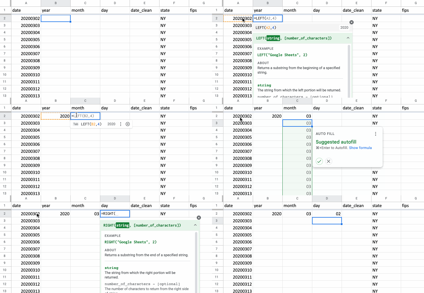
| year | month | day |
=LEFT(A2,4) |
=MID(A2,5,2) |
=RIGHT(A2,2) |
Filling down
So we’ve got row of good data. But what about the rest?
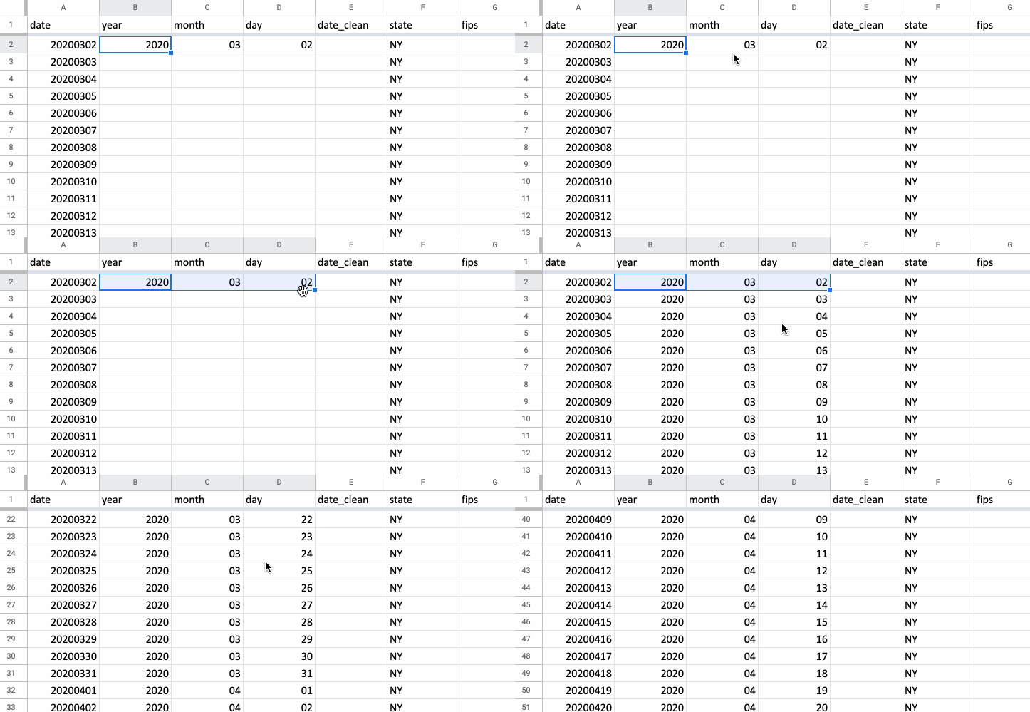
Instead of copying the formula hundreds of times, we can use an operation called fill instead. In this case, we’ll fill down – and because we’re using cell references, Sheets is smart enough to assume that we want to perform the same operation to the cell in the same relative location all the way down to the bottom of our data.
Use fill down by highlighting the three cells containing your formulas.
In the bottom right corner of the selection you highlighted, you’ll see a black square. Hover your cursor over it until the cursor turns into a black cross.
Double-click, and you’ll apply the fill down operation to all your rows.
Now we can reconstruct our date using the DATE function, which accepts as its three parameters a year, month and day.
=DATE(year, month, day)
Like you did with our other functions, use cell references to supply your arguments for your very first row of data. Then use the fill down operation to fill in the rest of the rows.
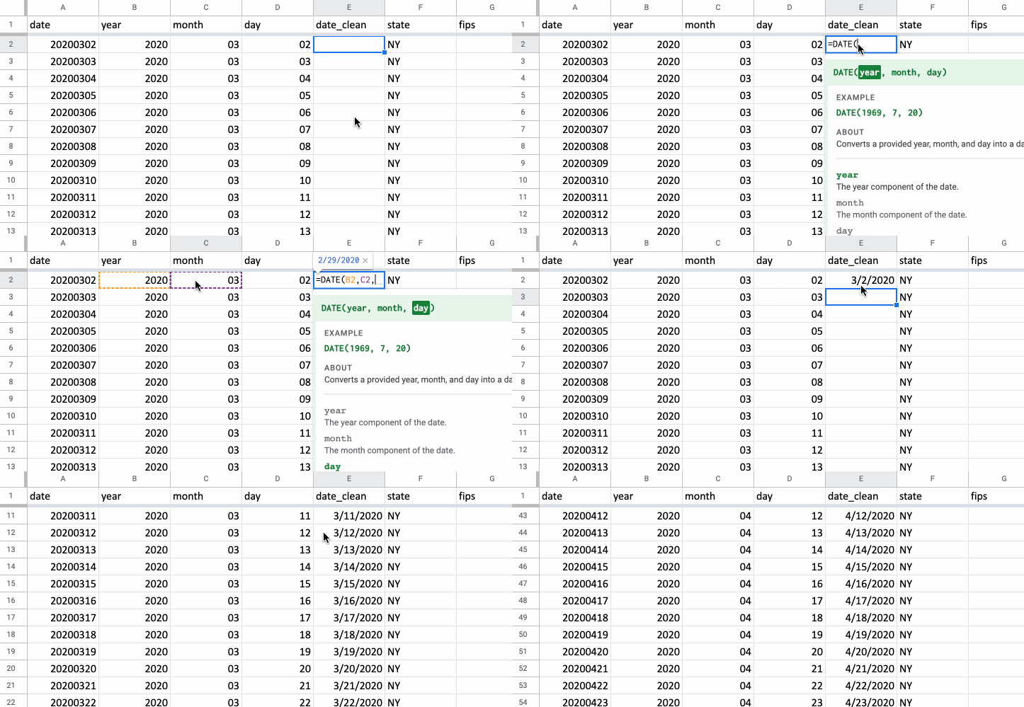
You may find that Sheets will prompt you with an option to “autofill” the rest of your rows, which gives you the same result.
There are often multiple ways to perform a task using spreadsheets!
Adding data with formulas
You probably noticed, just on the cursory look we’ve given the data so far, that some of the fields counting COVID-19 cases are cumulative. That constant growth might obscure some trends and story ideas we might find if were to look at spikes and slowdowns.
Let’s create two new columns – positive_new and positive_avg – at the end of our spreadsheet’s existing columns.
We’re going to use simple math to calculate the day-to-day changes.
But we need to be careful.
Unlike the previous functions, where we were performing column-wise operations that more or less wouldn’t be affected by the sorting and filtering, this next step is a row-wise operation.
If we sort the data into a different order, the formulas will recalculate and our values will change!
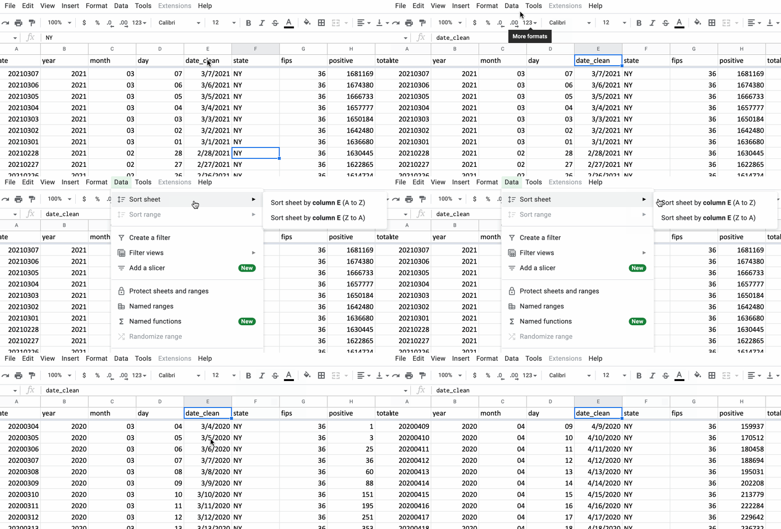
Start this process by sorting our dates in ascending (or oldest to newest) order.
Click on any cell in the date_clean column. Then use the menu bar to select Data > Sort sheet > Sort sheet by column E (A to Z).
With our data sorted, we can start generating our new figures.
We want to create a daily count of new cases by subtracting each row’s cases by the previous row’s cases – today’s count minus yesterday’s count. But where we previously built our new columns beginning with the first row of data, we actually have to start with day two this time.
Otherwise, we have no “yesterday” to compare with “today.”
In the second row of your new positive_new column (which is actually marked with a 3 because of the header), type an equal sign and click on the positive cell in the same row (H3). Type a minus sign, then click on the positive of the previous day (H2). Press enter.
=H3-H2
Nesting formulas
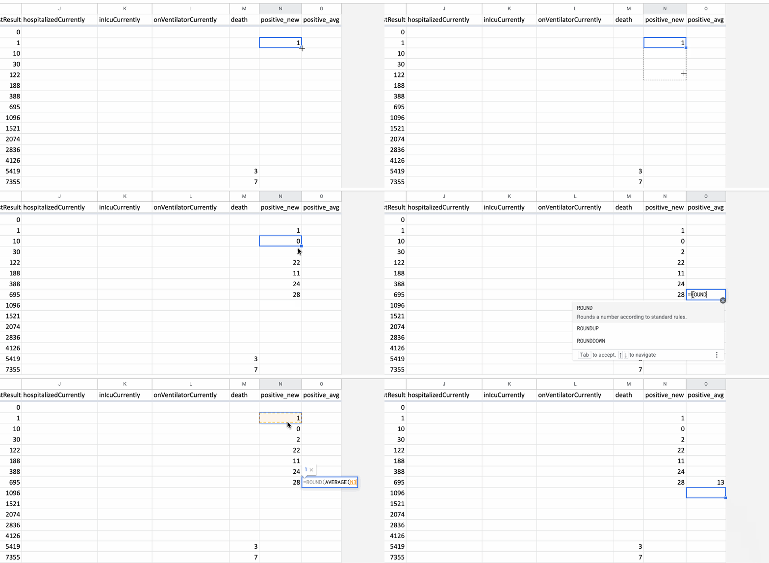
Don’t worry about filling down the whole column. Instead, click on the blue box in the bottom right corner of your positive_new cell and drag it down six more rows – giving you a total of seven entries.
We’ll worry about the rest of the rows later. For now, let’s focus on our positive_avg column.
What we want to calculate is a rolling average of new cases – in this case a seven-day average – that can help us flatten out the natural “spikiness” we’d expect from a daily count.
Why would the daily value be spiky?
Think about how the data is collected. Do people surge to test sites on different days of the week? Do weekend hours affect how quickly tests are processed and reported? These factors at the beginning stage of the data system can obscure meaning, so viewing both numbers – daily counts and a rolling average – might help us detect signals in the noise.
We can use the AVERAGE function to do the math, but we’re likely to get a bunch of decimals of precision that would muddy our analysis. So we’re also going to use the ROUND function to round the result of the average to the nearest whole number.
By nesting these formulas – one inside another – we can run both functions at once. Like so:
=ROUND(AVERAGE(values))
To the right of the seventh entry of your positive_new column, enter both functions and select the seven items in the adjoining positive_new column.
Pasting values only
You may notice, if you try the fill down trick from our previous steps, that nothing happens.
Why?
Notice that the adjoining death column has no data – the state hasn’t reported any COVID-19 related deaths as of March 2.
Sheets performs the fill down operation based on the number of rows in the adjoining columns. That’s why, in our other columns, it didn’t keep updating each row all the way down through our 700-odd blank rows.
We’ll have to fill down a slightly different way this time by highlighting all the cells we want to update.
If you want, you can do this by clicking that blue square in the corner of your positive_new cell and dragging aaaaaaallll the way down to the bottom of your sheet. But that’s annoying. And when your data gets bigger, it’s way too time consuming.
Instead, we’ll use a few keyboard shortcuts.
Click on any number in the death column. Then use CTRL + ↓ (PC) or CMD + ↓ (Mac) to jump down to the end of the sheet. If we mash the right arrow (→), we’ll pop over to the last blank row in the positive_new column.
Next, hold down SHIFT and hit the right arrow (→) to highlight the bottom-most cells of your positive_new and positive_avg columns.
Now hold down SHIFT + CTRL (PC) or SHIFT + CMD (Mac) and hit the up arrow (↑). This combination of shortkeys keys allows you to both collect ( SHIFT ) and jump ( CTRL/CMD ), highlighting all the cells up to your next non-blank entries.
Now press CTRL + D (PC) or CMD + D (Mac) – the keyboard shortcut for fill up.
Just like with fill down, you’ll see the formula you wrote up top copied and updated row by row.
One last thing we’ll need to do.
Remember the caution earlier about sorting with our new positive_new and positive_avg columns? We’re going to prevent ourselves from making that mistake.
Click on the letter column references at the top of your two columns (they should be N and O) to highlight them. Right click to bring up the mouse dialogue and click Copy.
Then right click again and click Paste special > Values only.
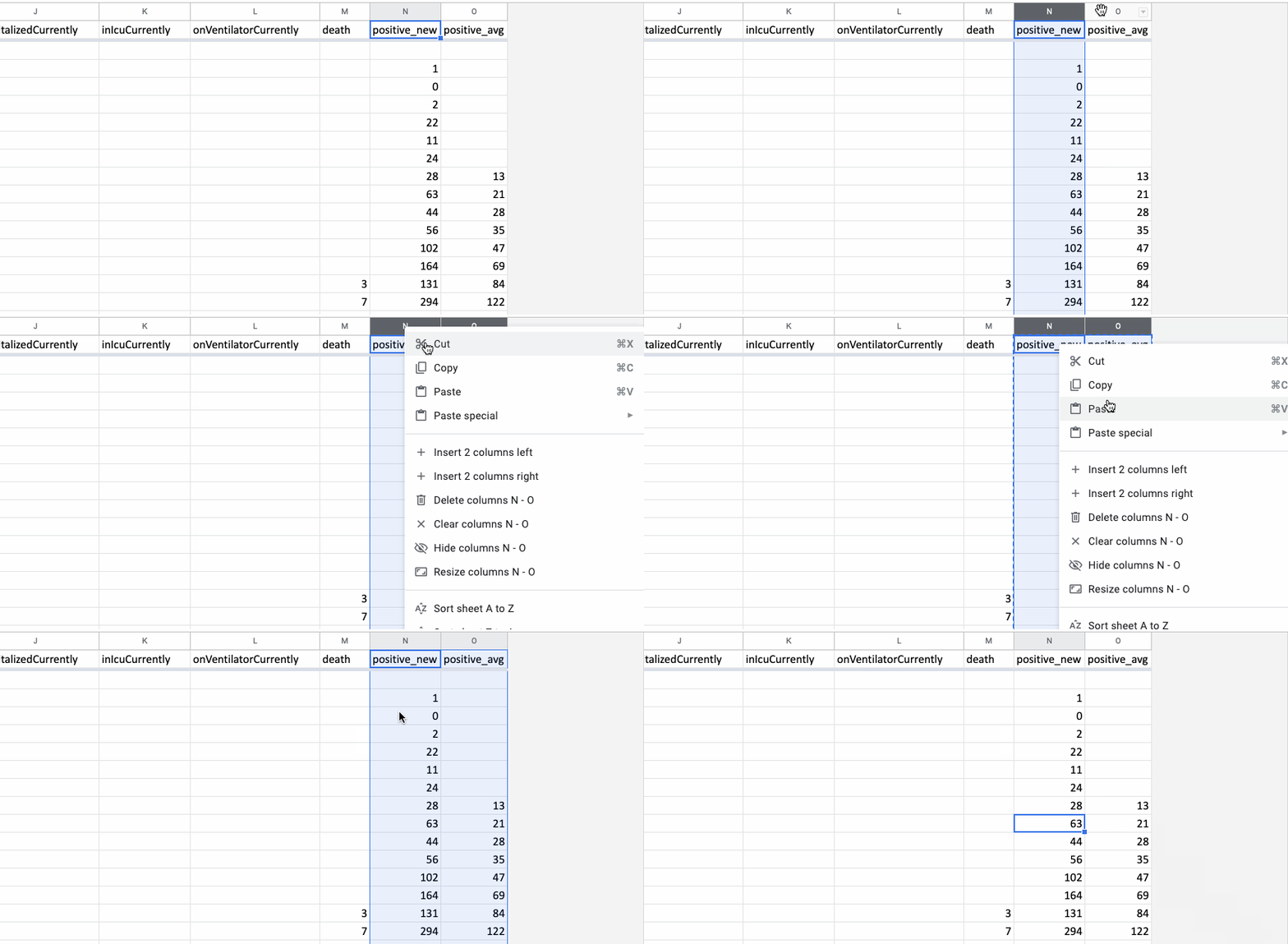
While it doesn’t look like anything changed, pasting these values overwrote all of our formulas.
And that’s a good thing! It means our figures can’t be overwritten if we sort.