Walkthrough: R and the Tidyverse

Total suggested time: 30 minutes

Using pre-built packages in R can dramatically expand its functionality. We’ll experiment with one common package in particular that can help us work with data.

Jump to a section

1. Starting an R project
2. Installing and importing packages
3. Downloading and importing data
4. Working with pipes
5. Sorting and filtering
6. Cleaning data with mutate
7. Adding columns based on existing data
8. Grouping by variables
9. Get the full script

Starting an R project

We’re going to organize our work in an R project, which keeps it all contained in a neat little folder on its own.

Start up RStudio and click File > New Project... in the top menu. You’ll be prompted to create a new project. If you’ve already got a folder for your work, you can choose Existing Directory and store the R project there. In our case, we’re going to click New Directory > New Project.

Give the directory a name (let’s go with covid_data) and place it somewhere we can find it again (that may be your Desktop or Documents folder).

Then click Create Project.

Now, when you create a new script with File > New File > R script, then ‘Save As…’, it will by default save to your project directory.

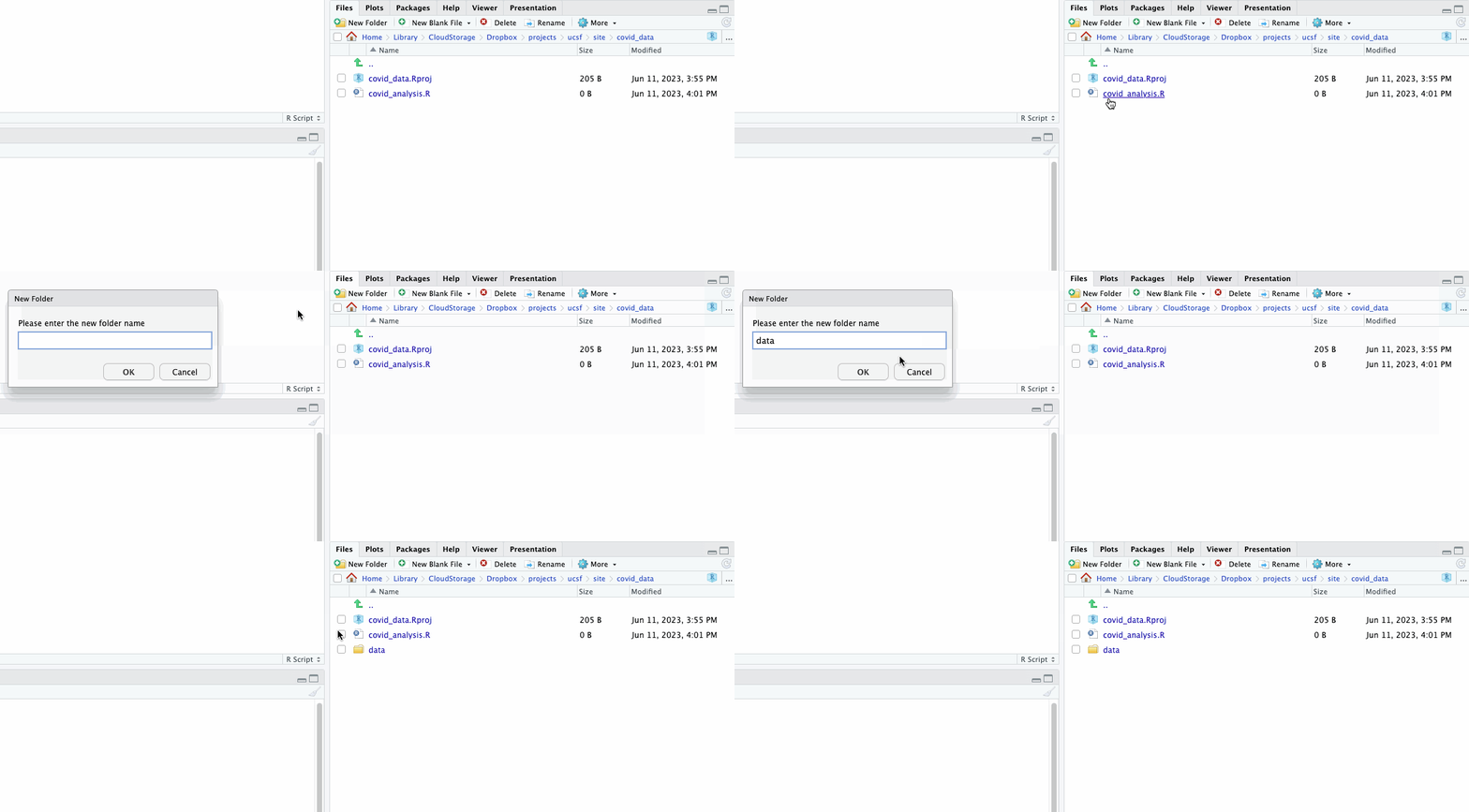
You can see all your project files in the “Files” pane in the bottom right.

You can also create new files and folders in the “Files” pane directly. Give it a try by creating a new folder in our directory we’ll name data.

Installing and importing packages

R has a lot of great, basic functionality built in. But an entire community of R developers has created a long list of packages that give R a wealth of additional tricks.

One of the most popular is the Tidyverse, a collection of packages designed for data science.

There are two steps to working with R packages:

1. Install the package – Required once for your machine
2. Import the package to your library - Required every time you start a new RStudio session

Like Excel and Sheets, R also uses functions to perform actions. We’ll use one of those functions – install.packages() – to install tidyverse now.

#install the tidyverse package
install.packages("tidyverse")

Execute the code by clicking the “Run” button at the top right of your script panel or by using the Command/Ctrl + Enter keyboard shortcut.

Then load them from our library.

#load our packages from our library into our workspace
library(tidyverse)

Downloading and importing data

We’ll be working with the COVID Tracking Project’s full data on testing and outcomes in the state of New York.

Download the CSV file here and save it to the data folder in the R project directory you created above.

If this looks familiar, you may remember it from the module on working with spreadsheets.

You can review the full data dictionary here.

We’re going to import the data on New York COVID cases using the read_csv() function from the Tidyverse package. This function loads comma-separated value files into a special type of R variable called a dataframe – basically just a table with rows and columns.

Here’s the command.

#load in our ny covid data
covid_ny <- read_csv('data/ny.csv')

Again, you can execute the code by clicking “Run” or with CMD + Enter.

This stores the data in a brand new dataframe variable named covid_ny.

Take note that in your “Environment” pane (by default in the top right), you should be able to see your dataframe with 371 rows (or observations) and 56 columns (or variables).

You can click on the dataset in your environment window to view it in a new tab in your “Source” pane, much like you would in Excel or some other spreadsheet software.

Working with pipes

For our analysis here, we’ll be using a Tidyverse specialty: the “pipe”.

Pipes – which look like this %>% – to chain together the output of functions from one line to the next line, allowing you to build complex operations with just a few lines of code.

As an example, let’s check to make sure we got all the data when we loaded it.

#how many rows do we have?
covid_ny %>% 
  nrow()

So we’ve got 371 rows. We should make sure none of the dates are repeated. For that, we’ll use the count() function, which accepts one or more fields from our dataframe and… well… counts them.

#make sure we've got 371 dates
covid_ny %>% 
  count(date)

Although you can take a look at the dataset itself by clicking on its name in the Environment pane, you might want to know more about the columns and their data types. For that, we can use the glimpse() function to view all your variables in a list, along with some information about their values.

#show me all the column names
covid_ny %>% 
  glimpse()

By the way: If we want to know more about a function – for example, the syntax or what sorts of options is has – we can prepend a question mark to trigger the “Help” tab.

#what's up with the count function?
?count()

Sorting and filtering

Just like with spreadsheets, we can use R to sort and filter.

For example, when did hospitalizations peak in New York?

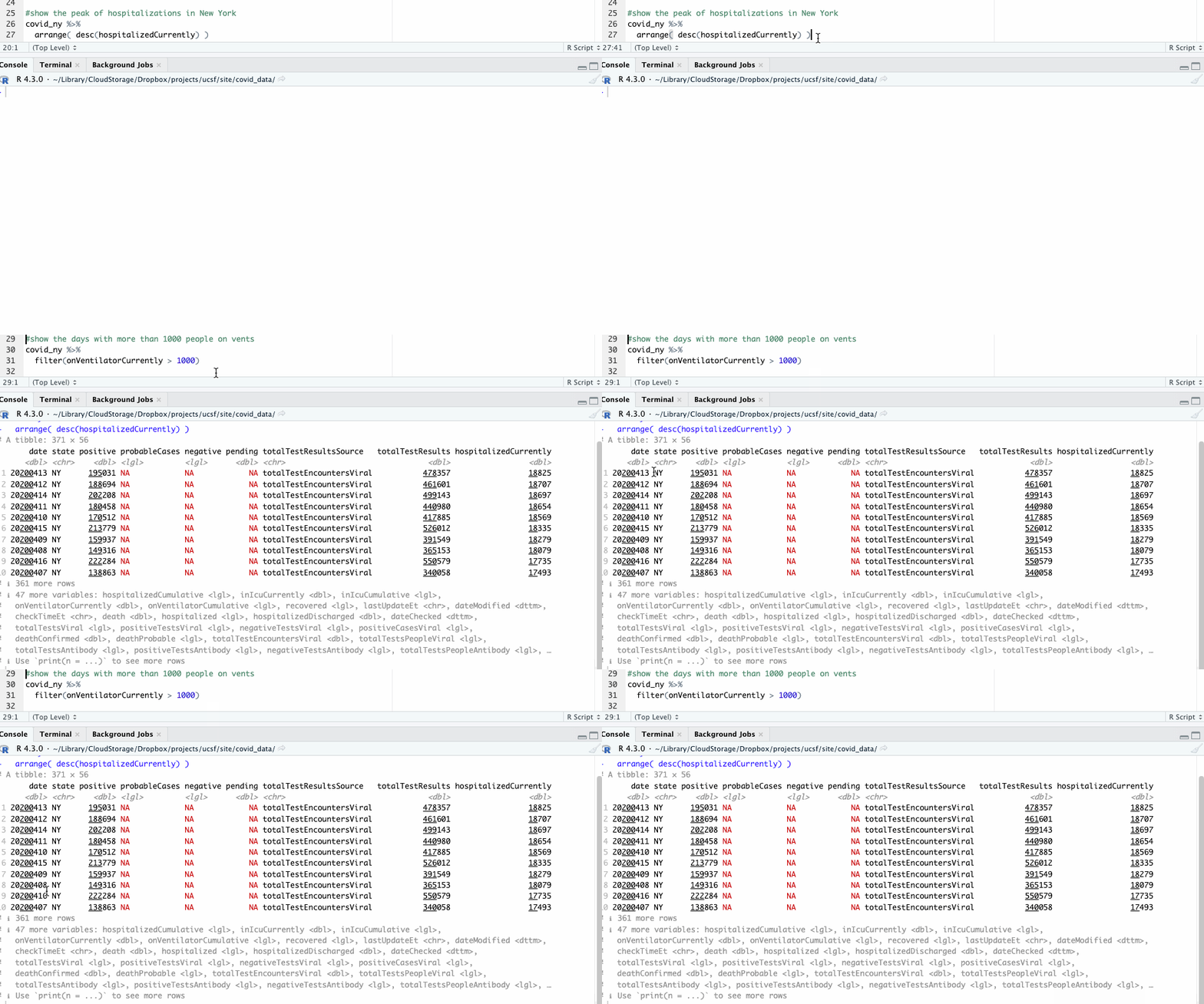
Find out using the arrange() function, where we’ll specify we want to see those currently hospitalized in descending order using the desc() function.

#show the peak of hospitalizations in New York
covid_ny %>% 
  arrange( desc(hospitalizedCurrently) )

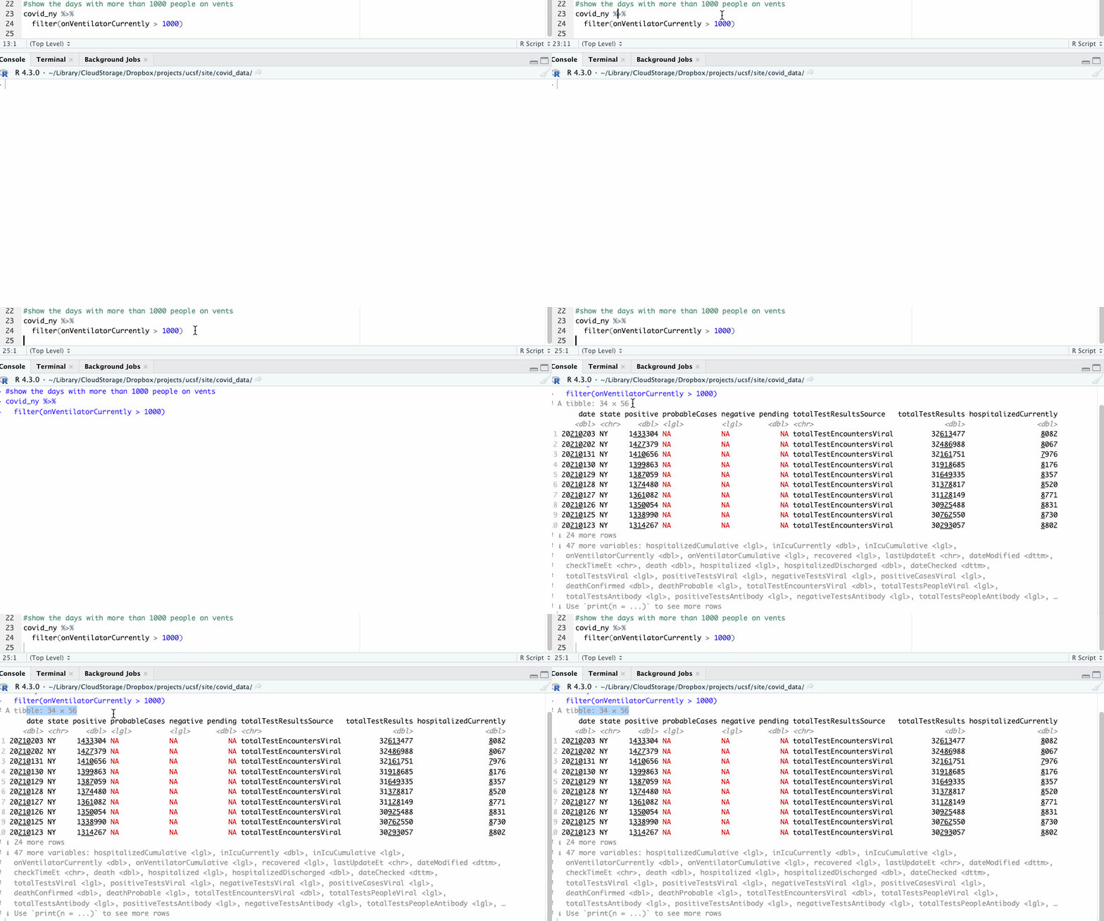
We can also filter our data by a certain condition, say, by days when there were more than 1,000 people on ventilators. We’ll use the filter() function for that.

#show the days with more than 1000 people on vents
covid_ny %>% 
  filter(onVentilatorCurrently > 1000)

By default, the output you see in the console will be truncated to 10 rows. You can see everything by piping your command to the view() function, which will open the results in a new tab.

#show the days with more than 1000 people on vents
#in a new tab to explore all of the results
covid_ny %>% 
  filter(onVentilatorCurrently > 1000) %>% 
  view()

Cleaning data with mutate

You may have noticed that the date field in our data isn’t quite right. One of the previous readouts even identified it as a “double” data type – a plain old number!

Let’s convert it to the right format with the mutate() function, which will add a column to our data.

We’ll call our new column date_clean, and we’ll use a few steps to get this right with the help of a few additional functions:

1. Convert the the numerical date to a string of characters with as.character
2. Convert the character date to a Date type variable with the as.Date function, specifying that the format is year (%Y), then month (%m), then day (%d).
3. Move the column to after the original date column using relocate

This time though, let’s assign the results to a new dataframe variable.

#convert the date and save to a new dataframe
covid_ny_clean <- covid_ny %>% #assign to new variable
  mutate(date_clean = as.character(date), #convert to character
         date_clean = as.Date(date_clean, format = '%Y%m%d')) %>% #convert to date format
  relocate(date_clean, .after = date) #change column order

Don’t see anything in your console? Don’t worry!

We assigned the output to a new variable, so you should see it appear in your Environment pane in the top right.

Adding columns based on existing data

When you ran a check with glimpse() earlier, you probably already noticed that many of the cumulative columns in our data also have columns calculating the day-to-day increase too.

That is, except for our number of hospitalizations, which for some reason is consistently 0.

Let’s fix that with mutate().

Because our data is organized so each row is a date, to calculate the change day over day, we’ll need to ask R for the previous day’s value to make our comparison. For that, we’ll use a handy function called lag().

First let’s ask R for the help file on the lag function.

#display an explanation of the lag function
?lag

Depending on how you’ve got your packages loaded, the Help pane may give you more than one option. Sometimes function names are repeated across different packages!

These two versions function in a similar way, but go ahead and click the option that reads: “Compute lagged or leading values”. There, we’ll see a detailed description of lag and its required parameters.

Description
Find the “previous” (lag()) or “next” (lead()) values in a vector. Useful for comparing values behind of or ahead of the current values.

When using lag() or lead(), order is important. So we’ll sort the data correctly before piping the output to our mutate() function.

#compute change in values for hospitalizations
covid_ny_clean <- covid_ny_clean %>% #overwrite our existing table
  arrange(date_clean) %>% #sort by ascending date
  mutate(hospitalizedIncrease = hospitalizedCurrently - lag(hospitalizedCurrently)) #calculate the change

If we view our dataset again, we can see the computed values now in the hospitalizedIncrease column.

Grouping by variables

Having more than a year’s worth of daily data is great. But we may have an easier time spotting trends if we examine the spread month to month.

We can do that by grouping our newly clean date column.

The Tidyverse makes this pretty easy with two functions: group_by() and summarize(). Much like they sound:

• group_by gathers all of your data into categories
• summarize performs an operation (like addition or average) across the entire category group.

The summarize() function doesn’t require group_by(). In fact, it’s an easy way to calculate descriptive statistics (average, median, maximum) on your whole dataset (which is technically just a single group).

#test out the summarize function
covid_ny_clean %>% 
  summarize(
    total_cases = sum(positiveIncrease), #calculate the total
    avg_increase = mean(positiveIncrease), #calculate the average
    median_increase = median(positiveIncrease), #calculate the median (middle value)
    max_increase = max(positiveIncrease) #calculate the maximum
  )

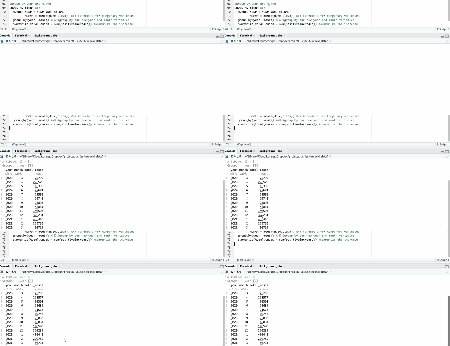
We’ll combine that functionality with another mutate() operation, where we’ll create a month and year variable to group on.

#group by year and month
covid_ny_clean %>%
  mutate(year = year(date_clean),
         month = month(date_clean)) %>% #create a few temporary variables
  group_by(year, month) %>% #group by our new year and month variables
  summarize(total_cases = sum(positiveIncrease)) #summarize the increase

Notice, by the way, that in this case we’re not overwriting any of our source data.

Like working with spreadsheet features like pivot tables, constructing these commands in R scripts allow us to run and rerun calculations in our data in a reproducible way, while leaving our original information intact.

Get the full script

Download the full script for this walkthrough here.